Losing money at video poker, with data science!
When I play video poker, I search for "corner" machines since someone once told me those are the best. Despite following this advice, I rarely cash in big. Although some psychological factors may lead the casino to loosen up the corner machines, my assumption is that all the video poker machines have the same odds. But what if they didn't? If the casino really had a few machines that favored the gambler, could I cash in?
Before analyzing some strategies, let's simplify our casino. Suppose that it costs $1 to play each machine, which pays $1 with some probability p. Since the casino can't be too tight if they want to attract gamblers, let's assume the optimal average payout across all machines is 0.48. Our toy casino only has two machines: one pays out 51 percent of the time and the other pays out 45 percent of the time, giving an average of 0.48.
Our goal is to distinguish between the good and the bad machine as fast as possible in order to take advantage of the machine that pays out 51 percent of the time.
We could try an A/B testing framework. As is standard, we would want 80 percent power, which means we need to have a large enough sample size to give us an 80 percent probability of rejecting the null hypothesis that the machines have the same underlying payoff. Then we could play the good machine until the casino kicked us out. To achieve 80 percent power given our machines' payoffs, we would need 2,174 total pulls, with half of them, or 1,087, coming from the bad machine. After this experiment, since our test has 80 percent power, we will identify and play the high paying machine 80 percent of the time, and in the other 20 percent, where we fail to detect a difference from the experiment, we will randomize between the machines.[1] Taken together, running the experiment costs $86.96.[2] But then we can take advantage of our knowledge. Our expected profit per pull is 0.8*($0.02) + 0.2*(-$0.04) = $0.008. For T - 2,174 exploitation steps, our total profit is: -$86.96 + (T-2,174)($0.008).
Rather than having a fixed number of samples from each machine before determining which is best, bandit algorithms, which get their name from slot machines, dynamically adapt their choice of what machine to play next based on the previous outcomes. Several bandit algorithms exist, but one of the most effective, and common, is the Upper Confidence Bound 1 (UCB1), which assumes payoffs are bounded between zero and one. At each time step, for each machine, we calculate the average of past pulls plus an upper confidence bound, which is based on the number of previous draws from that specific machine and our current time step. We then select the machine with the highest upper confidence bound, receive a payout, and repeat. This simple algorithm has near-optimal performance and protects against playing a wildly worse machine too many times because we only play a machine if its upper confidence bound is large, but since the confidence bound shrinks with each play, we quickly abandon bad machines.
However, unlike in the A/B testing case, we cannot easily calculate the expected profit, in part because the choices are made dynamically. Instead, we ran simulations to estimate expected profit. The figure below shows the cumulative profit after one thousand simulations, each containing 20,000 pulls. The chart shows the mean, 5th--95th percentiles of the UCB1 algorithm along with the expected profit from the A/B test.
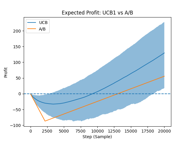
The figure above shows that the UCB1 algorithm typically experiences higher profit than the A/B test. Notice that the A/B test has two linear segments, one for the exploration phase, where it loses money, and one for exploitation, where it makes money. But the A/B test only chooses the correct machine with 80 percent probability, and never improves no matter how many draws it makes. The bandit algorithm, however, continuously improves. As it takes more samples, it plays the better machine more, leading its profits to diverge from the A/B testing strategy. The table below shows the cumulative profit at selected milestones, including breakeven points from the figure above.
| Step | UCB Mean Profit (5th–95th percentile) | A/B Expected Profit |
|---|---|---|
| 1,000 | -$20.23 (-$37.01 to -$5.01) | -$40.00 |
| 3,000 | -$32.09 (-$70.98 to $2.01) | -$80.35 |
| 6,000 | -$23.94 (-$83.98 to $26.42) | -$56.35 |
| 9,000 | -$2.50 (-$78.73 to $61.82) | -$32.35 |
| 9,268 | $0.00 (-$77.73 to $65.01) | -$30.21 |
| 12,000 | $28.07 (-$59.26 to $104.33) | -$8.35 |
| 13,045 | $40.25 (-$50.06 to $119.17) | $0.01 |
| 15,000 | $63.94 (-$33.52 to $150.52) | $15.65 |
| 20,000 | $129.57 ($17.82 to $227.83) | $55.65 |
The table illustrates that the bandit algorithm breaks even nearly 4,000 steps before the A/B test. Furthermore, as highlighted in the figure above, by continuously improving, the bandit algorithm makes nearly 2.5X more profit than the A/B testing strategy after 20,000 steps. In this casino, the bandit algorithm clearly dominates the A/B test.
But no matter the strategy, notice the number of pulls I would need to break even. Let's say I can play one hand every 5 seconds, or 12 hands a minute. That is 9,268/12 or 772 minutes, which is 12.8 hours of playing video poker. Using the A/B testing strategy, I would need 1,087 minutes, or 18.1 hours of playing these two machines just to break even. This shows that although we could profit over the long term, as Keynes said, that much video poker would leave us dead before cashing in.