Sources of Polling Error

• 08 November 2023
• polls

Pollsters and journalists often present polling results as being correct to within a plus or minus three percentage points, with 95 percent confidence. However, we often see election results fall outside this three percentage point error. In the 2020 election, for example, polls missed by an average of 4.5 percentage points at the national level. This post explores where this additional polling error comes from and how we should interpret polls in light of this additional error. As a quick note, since polls are surveys of respondents' vote preferences, I use the words polls and surveys synonymously.

Sampling Error: The Plus or Minus 3 Percent #

If we assume a three percent margin of error and we see a poll that says 54 percent of the respondents prefer Hans to Franz then we can be 95 percent confident that the true proportion of the population as a whole that prefers Hans lies somewhere between 51 and 57 percent. The "95 percent confident" means that if we ran our poll a million times, we would only see a result less than 51 percent or greater than 57 in only 5 percent of these polls.

The following bit of python code simulates this process. The code assumes you ask 1,000 people if they prefer Hans or Franz. If they prefer Hans, record a 1. Otherwise, record 0. We assume the true proportion of the population that prefers Hans a is 54 percent. This is one poll. We can now run this 10 thousand times and see how often the polls find support as either less than 51 percent or greater than 57 percent.

import numpy as np
population_pct=.54 # True value of the population
poll_sample_size = 1000 # poll 1000 people
test_draws = np.random.binomial(poll_sample_size, pop_pct, size=10_000)/poll_sample_size # sample from a binomial distribution; divide by n since we want a proportion

The plot below compares each of the 10 thousand samples from this distribution to what we would expect in theory. Notice that they are quite similar.

import numpy as np
from scipy import stats
import matplotlib.pyplot as plt

min_num_vot = 450
max_num_vote = 631

x = [int(i) for i in range(min_num_vot, max_num_vote)]
theoretical_distribution = stats.binom(n=poll_sample_size, p=pop_pct).pmf(x)
x_label = [i/poll_sample_size for i in x] # scale for plot, want a proportion, not raw count out of 1000

fig, ax = plt.subplots()

hist, bins, _ = ax.hist(test_draws, density=False, label='Samples', bins=10)

# scale pmf to match area in histogram; bin widths are scaled by 1000
scaled_pmf = theoretical_dist*np.sum(hist*np.diff(bins)*1000)
ax.plot(x_label, scaled_pmf, linestyle='--', label='True Distribution')
ax.set_title('Samples vs True Distribution')
ax.set_ylabel('Number of Polls')
ax.legend()

prop_outside_3_pct = np.sum(np.abs(test_draws-population_pct)>.03)/len(test_draws) # how many are outside 3%?
print(f'Proportion outside 3 percentage points: {prop_outside_3_pct: .2f}')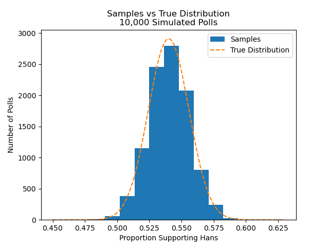

Proportion outside 3 percentage points:  0.057

The output shows that close to five percent of the estimates fell outside of plus or minus three percentage points of 54 percent, or about 95 percent were between 51 and 57 percent support for Hans. We see 5.7 percent, rather than 5 percent, of the estimate fell outside of 3 percent because the estimate's standard error, depends on both the number of people you poll (n) and the true proportion of the population that supports candidate A.^[1] But a sample size of 1000 generally gets close to 3 percent margins at 95 percent confidence.

The three percentage point error above occurs because we only take a sample of 1,000 from the population rather than measuring the whole thing. Randomness in who is sampled leads to deviations from the population's true value. However, sources other than sampling error generally cause polls and surveys to be off.

Bias: Who Answers Pollsters? #

In addition to sampling error, any error in a poll can be decomposed to two factors: bias and variance. Bias is how systematically wrong polls tend to be in a certain direction. For example, when polls all tend to overestimate their support for Franz, they are biased. Variance is the error in excess of the sampling error described above, but is not associated with any particular direction -- it can be either to favorable or too unfavorable to Franz. Typically, tools to reduce bias increase variance and vice-versa, this is the well-known bias-variance tradeoff.

A poll will be biased if one candidate's supporters are systematically less likely to respond to a pollster than their competitor's supporters. Conversely, sometimes a candidate's supporters may over-respond to polls relative to others. For example, they could be particularly excited about their candidate, or be eager to voice their displeasure at a scandal.

The simulation below shows what happens when one side's supporters are systematically less likely to respond to the pollster. We can then look at a simple method to adjust this bias assuming we have estimates on what group is under-responding.

For the simulation, assume the population is split in half between two groups: group A and group B. Group A will support Hans with a 44 percent probability, while group B will support Hans with a 64 percent probability. If both groups were equally likely to respond, we would expect to see an average of 54 percent support for Hans. However, let's assume group B will only respond to the pollster with a 25 percent probability; while everybody in group A responds to the pollster. In the simulation below, the pollster just needs to sample 1000 people. The pollster doesn't necessarily know what group each respondent belongs to, even though we will collect the groups in the code.

The code below simulates one pollster collecting this data.

a_vote_prob = .44
b_vote_prob = .64
b_response_prob = .25
results = []
group = []
poll_sample_size = 1000
i = 0
while i<poll_sample_size:
    a_vote = stats.bernoulli(a_vote_prob).rvs()
    results.append(a_vote)
    group.append('a')
    i+=1
    if i==poll_sample_size:
        break
    if stats.uniform().rvs()<=b_response_prob:
        b_vote = stats.bernoulli(b_vote_prob).rvs()
        results.append(b_vote)
        group.append('b')
        i+=1

The code above only simulates one poll. The following simulates 10 thousand different polls.

n_polls = 10_000
num_b_resps = stats.binom(poll_sample_size//2, p=b_response_prob).rvs(n_polls) # tried to get 500 of each group

num_a_resps = np.array([poll_sample_size - i for i in num_b_resps]) # Pollster needs 1000 respondents, depends on how many they get from b
a_resps = stats.binom(num_a_resps, a_vote_prob).rvs((1, n_polls)) # a responses
b_resps = stats.binom(num_b_resps, b_vote_prob).rvs((1, n_polls)) # b responses

biased_total = (a_resps + b_resps)[0]/poll_sample_size

## Collect weights, will discuss below
a_weight = a_prop_population/(num_a_resps/poll_sample_size) # Numerator is the proportion in the population
b_weight = b_prop_population/(num_b_resps/poll_sample_size)

ipw_weighted_total = (a_weight*a_resps + b_weight*b_resps)[0]/poll_sample_size

We can now plot what proportion of the population supports Hans according to each of these 10 thousand polls.

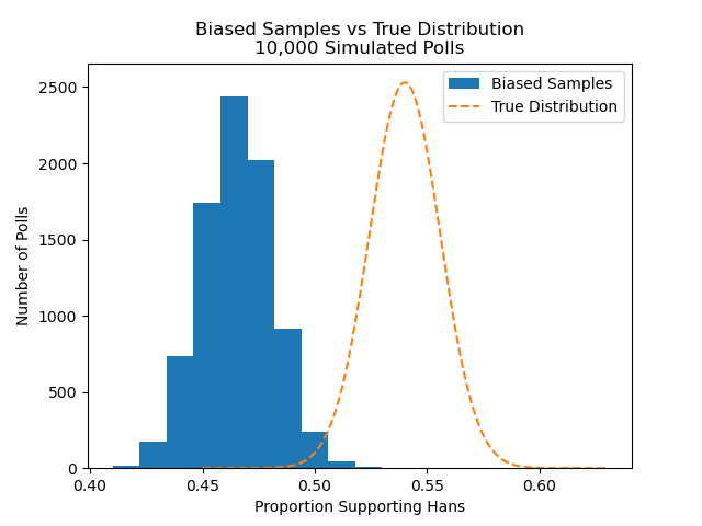
The plot below shows the polls are substantially biased against Hans' support. The average amount of support across all 10 thousand polls is 47 percent, rather than the true level of 54 percent. You can also notice very little overlap between the true distribution and the polls. If we run code to see how many of our samples are within three percent of the true value, we get the following:

Proportion outside 3 percent:  0.9976

In other words, only 24 out of the 10 thousand polls were within 3 percentage points of the true value. This would occur despite sampling error alone suggesting that 950 should have fallen within 3 percentage points of the true value. If we assumed a 3 percent margin of error, we could be fairly confident Franz would win.

From this example, we can see that substantial bias can result when one segment of the population does not respond to the poll and this segment also has different views than those more likely to respond. Fortunately, we can adjust for this bias, at least when we know who is under-responding.

Correcting Bias, Adding Variance #

The code above also included weights. Let's assume that the pollster knew the true distribution of groups A and B in the population, which we defined as 50/50. Let's also assume that the only factor that impacts how likely someone is to respond to the poll is what group they are in.

Although many techniques exist to correct for bias when you have group-level characteristics, we can use a simple one here: inverse probability weighting (IPW). Essentially, IPM increases the weight for each response for the group that was under-sampled and decreases the weight for each response in the group that was over-sampled.

The figure below shows the results we get if we adjust the biased draws above with IPW.

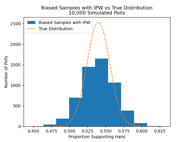
Although this distribution is centered close to the true value of 54 percent, notice that the samples are "wider" than the theoretical distribution. This means that each poll is noisier than expected. We can run code similar to the above to find what proportion falls outside +/- 3 percentage point from the correct value of .54:

Proportion outside 3 percent:  0.1964

After this bias correction, we now have nearly 20 percent of each pall falling outside of +/- 3 percentage point from the true value -- substantially more than the five percent we would expect from sampling error alone.

Unfortunately, pollster's efforts to adjust for bias often results in more variance. Because you may add substantial weight to a small number of respondents, the makeup of these particular respondents can cause poll results to fluctuate wildly. A notable example occured in 2016, when one person was weighted around 30 times as much as the average respondent. When this person was out of the sample Clinton led; when he was included Clinton trailed. This poll wasn't necessarily systematically pro or anti Clinton, but the inclusion of this one additional respondent made the poll's expected level of Clinton support to vary far beyond what sampling error alone would have us believe.

How Does This Impact Professional Polls? #

A 2018 paper by Shirani-Mehr and coauthors ^[2] analyzed US gubernatorial, senatorial, and presidential election polls in the final three weeks of the campaign between 1998 and 2014 with the goal of disentangling the amount of bias and variance in the polls. They find that, on average, bias is about 2 percentage points. This bias isn't systematically for or against either party but fluctuates at random -- if there was a correlation with political party, it could be adjusted for.

Additionally, the paper finds that variance is about 1.5 percentage points more than we would expect from sampling error alone. The authors speculate this is due to the methods pollsters use to account for bias. Taken together, the additional bias and variance suggests that rather than assuming polls are accurate to within +/- 3 percentage points, we should really assume they are accurate to within +/- 6 to 7 percentage points. This spread would have covered many of the polls in 2020, the biggest polling miss since 1980, where the average poll was off by 5.1 percent at the state level.

In addition to assuming the margin of error is much larger than 3 percent -- which doesn't even make sense in theory since we know there is more than sampling error leaking into polls -- we should think hard about who decides to respond to a poll when interpreting its results, since polls can fail drastically if biasness isn't accounted for.

A recent poll following Israel's invasion of Gaza showed a surprisingly large number of Gen-Z respondents believed Hamas' murder of civilians was justified. This poll was taken as protests broke out across the country against Israel's invasion. During the 2020 George Floyd protests, protestors were systematically younger than Americans as a whole. If these age trends continued, the protests against Israel likely skewed Gen-Z. Protesting may also fires these activists up for their cause, making them more likely to respond to a pollster. If these protestors are also more likely to agree with more extreme statements -- perhaps just being caught in the moment -- then the amount of support for Hamas' use of violence would be drastically inflated. We can try to look toward other indicators to determine how plausible this explanation is. Or perhaps this poll is solid and more than 50 percent of young people support Hamas' act.

Footnotes #

• Next: Can Biden Make Bibi Balk?